Computing alpha and beta parameters for ILs
Introduction
The following outlines the procedure for the computation of EPnuc and ΔE(HCN) for the prediction of α and ΔE(HF) and Δr(HF) for the prediction of β. The [C4C1im]+ cation and [BF4]- anion will be used here to illustrate the processes for α and β respectively. All calculations for these examples can be run on a standard laptop computer.
The calculations have been carried out using Gaussian and the associated visualization package Gaussview. If you are unfamiliar with Gaussian and Gaussview there is a short introduction to building a molecule and running an optimisation here: simple gaussian lab (which is part of a 3rd year UG computational lab course)
It is well worth your while to read the Gaussview help and to have a go at the associated "Basic Molecule Building" tutorials. (Ignore the advanced features for now)
We highly recommend Exploring Chemistry with Electronic Structure Methods: A Guide to Using Gaussian, by James B. Foresman and Eleen Frisch.
Here are some useful links:
- my simple instructions on how to start using gaussian: simple gaussian lab
- Gaussian Website
- List of keywords used in Gaussian
- the Basis Set Exchange for basis sets and pseudo-potentials
The following instructions assume you have some basic knowledge of running calculations (ie have at the very least completed my on-line lab above)
The calculations shown here use the B3LYP/6-311+g(d,p) method and basis set. Although other DFT functionals, basis sets, or higher methods could potentially be employed, for a meaningful comparison across any series of cations or anions the level of theory used should be consistent.
Also, if you want to use the linear relationships published in the paper you must carry out your calculations at the same level that the original relationship was established. For example, you will compute EPnuc for your cation and then use this value in the following equation, α=5.153*EPnuc +5.136, to make a qualitative estimate of α. A similar association holds for the other parameters used to determine α or β.
Optimisation
Before the selected properties can be computed, all cations and anions must first be optimised and confirmed as minima on their respective potential energy surfaces via frequency analysis. While these can be run as a single job, it is best to first optimise and then run the frequency analysis in two seperate jobs. This way if your optimisation does not work the first time or is not complete, you have not wasted computer resources.
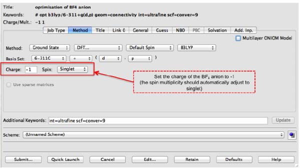
All calculations here have been performed using B3LYP/6-311+g(d,p) with the additional keywords int=ultrafine and scf=conver=9. You will need to set up your calculations with these options, they improve the convergence criteria and integration grid over the Gaussian defaults. As we are working with ions, it is important to remember to adjust the charge of the system accordingly.
Below is an image of what your setup-up should look like in gaussview.
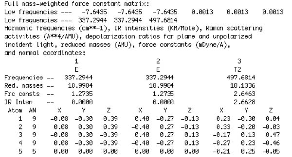
At the B3LYP/6-311+g(d,p) level, we would normally expect the six lowest frequencies to be within, or close to, +/- 10cm-1. An extract from a completed frequency job is provided below.