
Viewing and Understanding your Optimised NH3 output
- Your *.log file should be open, but if you have closed it you can open it again by choosing "File and open" in gaussview. Navigate to D: drive folder and open your log file.
- What if you cannot find the *.log file from inside gaussview? The file should be there however, sometimes silly microsoft does not give the .log extension. So navigate from the desktop of your PC to find the file you think is the *.log file (in your folder) and click on it choosing open in gaussview. If this doesn't work you might need to switch on the filename extensions in Windows.
- If something has gone wrong ask a demonstrator for some help, if there is time they will help you work out what went wrong. If there is not enough time for this, goto the end of this page and download some pre-prepared files!
- To obtain general information about the job click on the results tab at the top and choose "Summary". This will open a window that lists important information about your calculation.

- The summary contains information which is important when writing reports or papers that include theoretical results. This kind of information is equivalent to recording the concentration of your reactants or the temperature of your reflux etc.
- Find out some geometric information
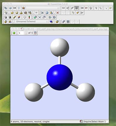
- on the commands palette click on the button with a question-mark in front of a ruler. This is the inquiry button and will tell you bond distances if you click on two atoms, and bond angles if you click on three atoms
- use the inquiry button to find out optimised bond distances and angles.
- some important conceptual things to know about how the various programs integrate.
- Gaussian "runs" the jobs (ie does all the number crunching)
- Gaussview is a separate program which is used to create and edit files used by Gaussian.
- When you submit a job you or Gaussview makes a *.gjf file and when you look at the output you or Gaussview is looking at a *.log file
- Gaussian also makes a third file, where it stores information in a "machine only readable format" these are called checkpoint files and have the file extension *.chk. Sometimes we will also use Gaussview to process information in the *.chk file for us to view graphically, like the molecular orbitals.
- Now we are going to look at the "real" output, the file that Gaussian generates. This is a purely text based file, Gaussview is an interface that takes information from this file and presents it to you graphically. Sometimes we want information that Gaussview cannot process and so we must look directly at the file output by the program Gaussian. This also allows us to double check the job has optimised successfully

- There is more than one way to access this file, you can click on the "view file" button in the summary (see above), or you can click on the results tab at the top and choose "View File ...".
- This file is the "real" output, a text based *.log file. Scroll through the file, if you are interested the deomonstrators can tell you more about the contents.
- Now check that your job has really converged, go to the end of the file and move backwards until you find the final set of forces and displacements, it should look something like this:
Item Value Threshold Converged? Maximum Force 0.000005 0.000450 YES RMS Force 0.000003 0.000300 YES Maximum Displacement 0.000012 0.001800 YES RMS Displacement 0.000008 0.001200 YES Predicted change in Energy=-9.075171D-11 Optimization completed. -- Stationary point found. ---------------------------- ! Optimized Parameters ! ! (Angstroms and Degrees) ! -------------------------- -------------------------- ! Name Definition Value Derivative Info. ! -------------------------------------------------------------------------------- ! R1 R(1,2) 1.018 -DE/DX = 0.0 ! ! R2 R(1,3) 1.018 -DE/DX = 0.0 ! ! R3 R(1,4) 1.018 -DE/DX = 0.0 ! ! A1 A(2,1,3) 105.7463 -DE/DX = 0.0 ! ! A2 A(2,1,4) 105.7463 -DE/DX = 0.0 ! ! A3 A(3,1,4) 105.7463 -DE/DX = 0.0 ! ! D1 D(2,1,4,3) -111.867 -DE/DX = 0.0 ! -------------------------------------------------------------------------------- GradGradGradGradGradGradGradGradGradGradGradGradGradGradGradGradGradGrad - the important information is in the part below "Item" the "YES" under Converged tells us that job has successfully converged.
- The computer never gets to exactly zero because of rounding errors, so we apply a threshold
- Information from a calculation is physically meaningful ONLY if the molecule is optimised. Thus optimisation is always the first step to examining the structure and electronic distribution (bonding) within a molecule.
- Check that your molecule is fully optimised! If not ask a demonstrator to take a look to help figure out went wrong. Every problem is a learning experience and deepens your understanding.
- Files for if something has gone wrong
- BF3(CF3) logfile CF3BF3_B3LYP_631Gdp_fopt.log
and checkpoint file CF3BF3_B3LYP_631Gdp_fopt.fchk - SO3(CF3) logfile OTf_B3LYP_631Gdp_fopt.log
and checkpoint file OTf_B3LYP_631Gdp_fopt.fchk
- BF3(CF3) logfile CF3BF3_B3LYP_631Gdp_fopt.log
You now have an optimised geometry we can examine other properties of the molecule
- When you are ready move onto the next step