Moleuclar Orbitals
- You have already started learning about Molecular Orbital (MO) theory, and you have a number of courses that cover different aspects of MO theory from the mathematics through to qualitative MO diagrams. MO theory is also used in organic steroelectronics and to describe transition metal ligand bonding
- Open the *.chk file (not the *.log file!) for final optimised NH3
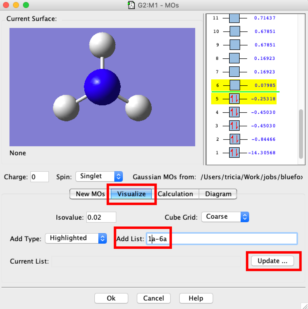
- Then from the "Tools" pulldown menu, choose "MOs"
- A MO window should open. In the new window select the "Visualize" tab and then in the box "Add List" type "1a-6a", and click on Update. What will happen next is that gaussview will read information off the checkpoint file and covert this into the molecular orbitals 1-6 for you to visualise. Be patient, this requires quite a bit of number-crunching and may take up to 10min. The larger the number of MOs to compute the longer this will take.
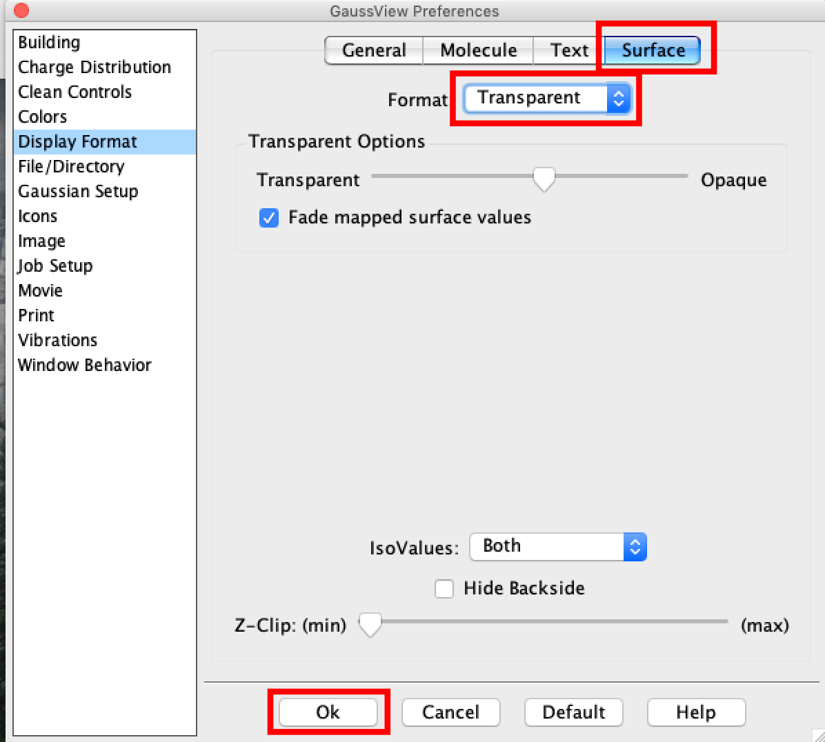
- While you wait, we want to set the surfaces to appear as transparent, this makes the MOs easier to interpret as you can see the atomic nuclei. Click on the Gaussview tab (top-right) select "Preferences" a new window will open. In the new window select "Display Format" click on the "Surface" button and then select "Transparent" from the pulldown menu. Once done click the "OK" button.
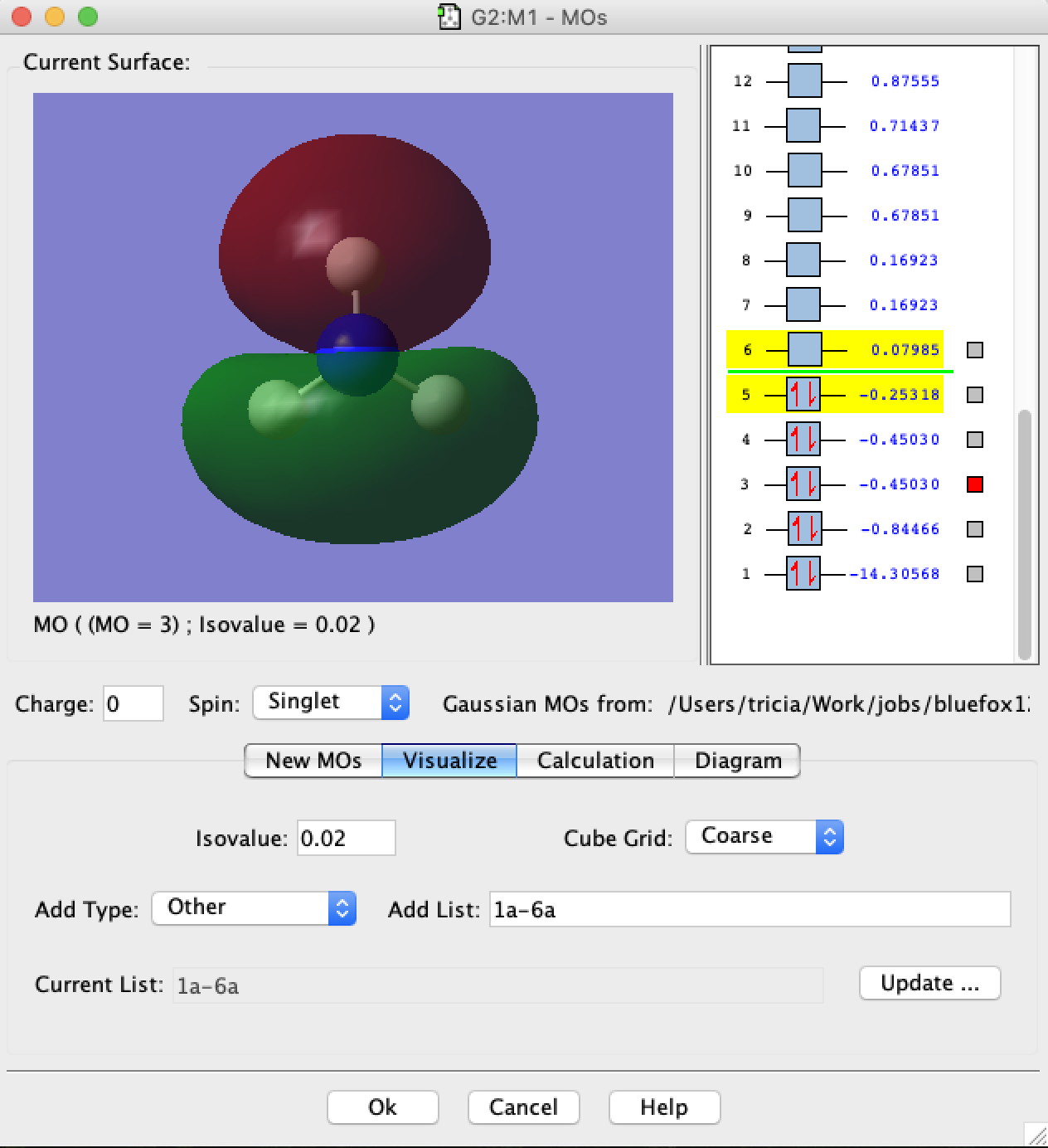
- Once the MOs are computed you should step through each of the MOs from number 1 through to the LUMO. The deep MOs determine the bonds that form in a molecule, the HOMO and LUMO determine the reactivity of the molecule.
- You could also look at the higher energy MOs above the LUMO, however their shapes are not as reliable as those of the bonding MOs particularly the higher energy ones. When you get to your quantum mechanics course you will learn that this is because the SCF procedure only variationally optimises the occupied orbtials. So in terms of the mathematics the way we arrive at the un-occupied MOs is not as robust.
- Spend some time compare your computed real MOs to those obtained by forming a valence MO diagram as given below. The grey levels represent the orbitals before mixing.
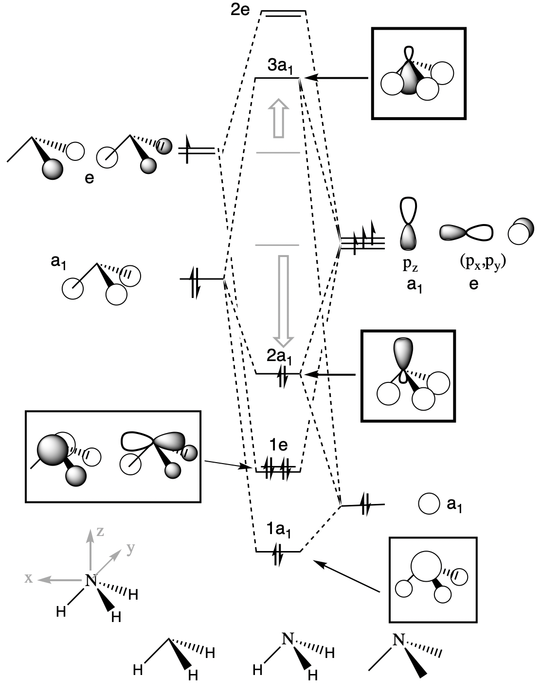
- MO1 from the calculation is the core 1s AO on the N atom (core orbitals do not appear on a valence MO diagram)
- MO2 from the calculation is the 1a1 MO of the MO-diagram, this is a totally symmetric, all in phase, bonding MO
- MO3 and MO4 from the calculation are degenerate and correspond to the 1e MOs of the MO-diagram, notice the good overlap between the N pAO lobes and the sAOs on the H-atoms.
- MO5 from the calculation is the 2a1 MO of the MO-diagram, and the HOMO, this MO demonstrates significant orbital mixing. Formally this orbital is the "lone-pair" from hybridization or VSEPR theory (Valence shell electron pair repulsion theory), notice that there is not actually much "lone pair" character to this orbital. Bonding in NH3 is an example of one of the (many!) places where traditional bonding theory breaks down and modern MO theory should be used
- MO6 from the calculation is the 3a1 MO of the MO-diagram, and the LUMO, this orbital is the antibonding partner of the mixed-HOMO. Notice the phase change from the outer to the inner part of the MO. This means a node occurs along the N-H bond, making this an antibonding MO close to the N nucleus. But notice also that there is positive overlap outside of the N-H bond region, making this MO bonding far from the N nucleus.
- Overall you can see that MO theory gives a very good first estimate of the MOs computed using the Schrodinger equation!
Now you have finished the "demonstration" section of the mini-lab, it is time to start work on your assignment molecule.