Optimising a Molecule of NH₃

• if it is not already the front window, bring the window with your NH₃ molecule to the front.
• now we are ready to set up the commands that tell the program how to do the calculation, we tell it
  • the method: B3LYP
  • the basis set: 6-31G(d,p)
  • and what type of calculation to do: OPTF (optimise and frequency analysis)
• The method B3LYP determines the type of approximations that are made in solving the Schrödinger equation.
• The basis set determines the accuracy, 6-31G(d,p) has a medium level accuracy, using this basis set means the calculations should be quick.
• In carrying out an optimization we are determining the optimum position of the nuclei for a given electronic configuration, this is the first step for any quantum chemical calculation.
• Depending on the gaussview set-up some of these options may be pre-set for you or you may have to select them yourself, you can also explore the buttons and options but please come back to the defaults
• We are also going to add a few extra commands as well to allow us to investigate the vibrational modes and electronic structure of the optimised molecule.
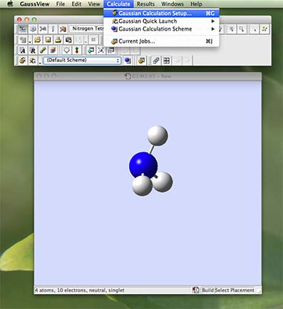
• From the main menu along the top of the screen (in gaussview) choose "Calculation" and then choose "Gaussian Calculation Setup...":

  

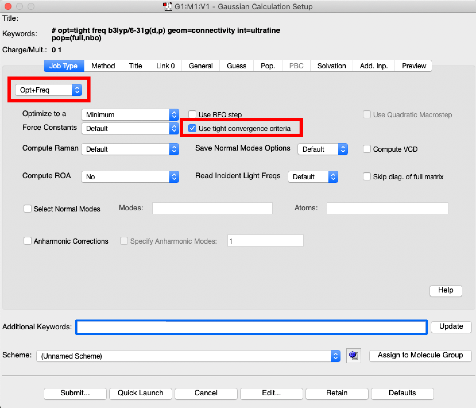
• a new palette will appear the calculation palette. It opens with the "job type" tab open. If the default is not set to "opt+freq" use the pull down menu to choose "opt+freq". This command requests that the calculation carry out an optimisation and then vibrational analysis. In addition you need to tick the "use tight optimisation criteria box".

  

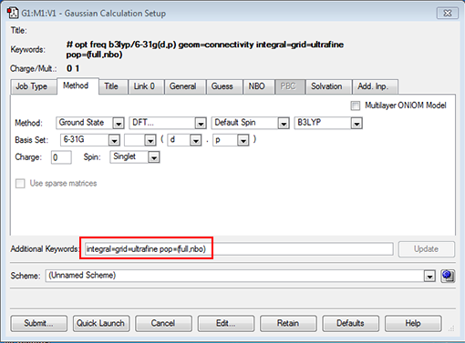
• next click on the "method" tab to open it, the default should be B3LYP for the method and 6-31G(d,p) for the basis set. There is also some other information in the "Additional Keywords" section this should say int=ultrafine OR integral=grid=ultrafine (these are just 2 ways of setting this option), this option relates to how accurately the electronic density is computed, we want it to be computed on an ultrafine integration grid.

  

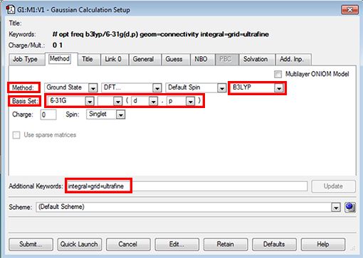
• If you don't see expected defaults then you can set the options yourself:
  • use the pull down menu under "Hartree-Fock" to pick "DFT"
  • find the pull-down menu "LSDA" and choose "B3LYP"
  • in basis set choose 6-31G in the first button
  • in basis set leave the 2nd button, but in the 3rd button choose "d" and in the 4th button choose "p"
  • type into the "additional keywords" section: integral=grid=ultrafine
• We want to add two more commands, the first NBO will ask the code to run a population analysis so the atomic charges are calculated and the second pop=full to record all the MOs so we can visualise them (the main objective of this lab). Type into the additional keywords section "pop=(full,nbo)" as shown below:

  

• We should also add a title for your job, so under the "title" tab type in something descriptive about the job I used "nh3 optimisation".
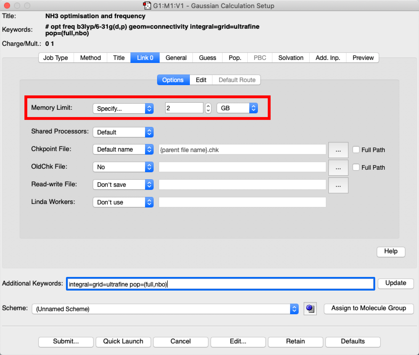
• Last and very important we need to set the amount of memory your job is allowed to use. Select "specify" on the pulldown menu and set this to 2 GB as shown below:

  

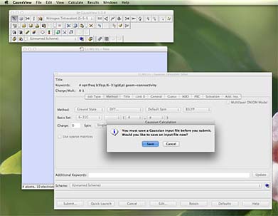
• Now you are ready to go! Press submit (button is in the bottom left of the palette)
• a new window will pop-up and telling you that you must save the file first, press "save":

  

• a new window will then pop-up and ask you for a file name.
  • first navigate to the D: drive where we will save the file, or you could save to a flash drive. Do NOT save onto the C:drive
  • linux does not like spaces in filenames NO SPACES in filenames use an underline "_" where you would use a space
  • include your initials in your filename
  • until you are experienced, remembering what is in every file can be difficult, give your file a short but descriptive name
  • for example, my initials are PH, this is a nh3 molecule and we are doing an optimisation, so I would name my file
  
  
  PH_nh3_opt.gjf
  
• a new window will then pop-up and ask you if you want to submit the job, press submit!
• close the molecule window, this is important as the "finished" molecule will look very similar to your starting one and many students accidentally take the wrong molecule in subsequent sections!
• a new window will then pop-up and ask you for a file name, navigate to your selected folder and save your input file. It is important to give your file a descriptive name otherwise after running a few jobs you will forget which one is which. For example "Firstname_Lastname_nh3_optf_pop.gjf" where Firstname is your first name and Lastname is your last name, then we add some text which identifies the molecule, and lastly what kind of job it is. Don't forget to use "underscore" instead of spaces because spaces have a special meaning in unix.
• a new window will then pop-up and ask you if you want to submit the job, press submit!
• close the molecule window, this is important as the "finished" molecule will look very similar to your starting one and many students accidentally take the wrong molecule in subsequent sections!
• You might have time to use the job manager, or your job may finish so quickly it is gone in a flash. To look at the running jobs, click on the "calculate" tab at the top, select the "running jobs" and you should see something like the top window below. Then if you click on "Stream Output File" you can see information printed to your output file (called a *.log file) as it is running! This is shown in the second window below:

  

• after a small amount of time a window should pop-up saying the job is completed, you want to open the *.log file. (The time your job takes to run will vary depending on how efficient your computer and network are, if you are waiting any more than 5min ask a demonstrator!)

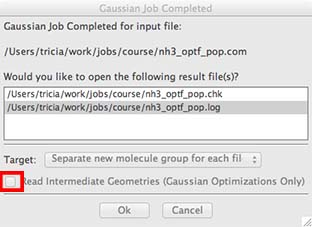
  You should also select the "Read Intermediate Geometries" box as well.

  

• the log (*.log) file contains information that is directly human readable, the checkpoint file (*.chk) contains information in binary that is only computer readable. Gausview reads these files and then graphically represents the information in them.
• When using gaussview it can matter which one you look at, use the *.log file normally, but when you want to visualise molecular orbitals use the *.chk file (more about this shortly!)

• This is your optimised NH₃ molecule!

• Now move onto the next step